1.   Introduction

3D generative modeling has made great strides via gravitating towards neural scene representations, which boast unprecedented photo-realism. Generative models^[1-5] can now draw class-specific scenes (e.g., cars and portraits), offering a glimpse into the boundless universe in the virtual. Yet an obvious question is how we can go beyond class-specific scenes, and replicate the success with general natural scenes ¹, creating at scale diverse scenes of more sorts. This work presents an attempt towards answering this question.

Another key that boosted the field is differentiable projection techniques that enable training on only 2D images, bypassing the explicit need for collecting 3D models. However, collecting tons of homogeneous images for each scene type ad hoc is cumbersome, and would become prohibitive when the scene type varies dynamically. Herein, our key observation is that general natural scenes often contain many similar constituents whose geometry, appearance, and spatial arrangements follow some clear patterns, while exhibiting rich variations over different regions. Therefore we propose to train on a single general natural scene, which builds upon recent success with differentiable rendering, particularly to learn the 3D internal distribution from its observation images.

To this end, we present SinGRAV, for a generative radiance volume learned to synthesize variations from images of a single general natural scene. Training with a single scene necessitates learning the internal statistics, which triggers a design choice of the scene representation with locality modeling in SinGRAV. Besides, different from object-centric scenes as in [1, 3, 4] or image generation^{[6, 7]}, plausible geometric arrangements are vital to 3D scene generation. Therefore, key designs are dedicated to improving the spatial arrangement plausibility, without significantly increasing the computational overhead.

Specifically, the core of SinGRAV is to learn from local regions via localizing the training. As our supervision comes from purely 2D observations, learning internal distributions consequently grounds SinGRAV on the assumption that multi-view observations share a consistent internal distribution for learning. This can be simply realized by capturing images with cameras at roughly uniform distances to the scene, e.g., with drones for outdoor scenes. On the other hand, multi-layer perceptron (MLP)-based representations tend to synthesize holistically and perform better at modeling global patterns over local ones^[8], as also revealed in our ablation studies. Hence, we resort to convolutional operations, which generate discrete radiance volumes from noise volumes with limited receptive fields, for learning local properties over a confined spatial extent, granting better out-of-distribution generation in terms of global configuration. Moreover, we adopt a multi-scale architecture containing a pyramid of convolutional GANs to capture the internal distribution at various scales, alleviating the notorious mode-collapse issue. This is similar in spirit to [6]; however, important designs must be incorporated to efficiently and effectively improve the plausibility of the spatial arrangement of the generated 3D scene. Specifically, we found that coarser scales produce highly implausible geometric structures, which cannot be easily distinguished by discriminators operating on the renderings with limited receptive fields. Our remedy is to use a combination of 1) the spatial inductive bias injected at the coarsest scale, and 2) the joint discrimination on the geometric depth map, which is a byproduct from reconstructing the input scene and also the volume rendering technique.

To validate the proposed framework, we collect a dataset containing various example scenes, and conduct comprehensive investigations. We demonstrate that SinGRAV enables us to easily generate plausible variations of an input scene in large quantities and varieties, which is exemplified by a subset of the results showcased in Fig.1. To evaluate the plausibility of generated scenes, we compare the observed multi-view images from the generated scenes against those from the given exemplar scene. And performance comparisons are made to state-of-the-art generative neural scene models. We also extensively investigate each key design choice for inspiring more future research. Finally, we show the versatility of SinGRAV through its use in a series of applications, spanning 3D scene editing, composition, and animation.

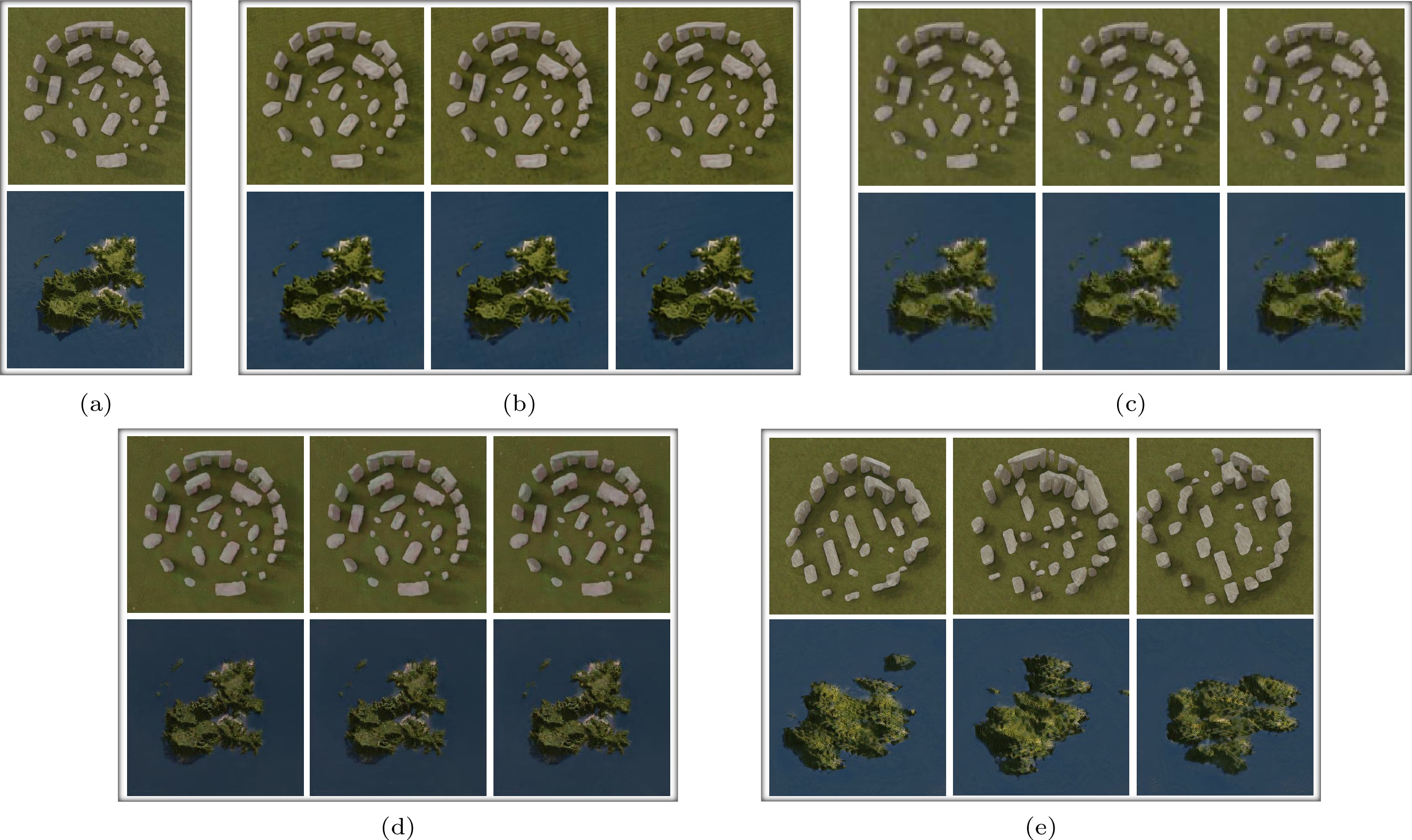
Figure  1.  Scene generation results and application results. (a) Three views of the training scenes. (b) Randomly generated scenes from the proposed framework SinGRAV. (c) Results for object removal. (d) Results for duplicating an object. (e) Results for scene composition. Note how the global and object configurations vary in generated scenes shown in (b) yet still resembles the original training scene.

下载: 全尺寸图片 幻灯片

2.   Related Work

Neural Scene Representation and Rendering. In recent years, neural scene representations have been the de facto infrastructure in several tasks, including representing shapes^[9-13], novel view synthesis^[14-16], and 3D generative modeling^{[1-5, 17, 18]}. Paired with differentiable projection functions, the geometry and appearance of the underlying scene can be optimized based on the error derived from the downstream supervision signals. [9-12, 19] adopt neural implicit fields to represent 3D shapes and attain highly detailed geometries. On the other hand, [16, 20, 21] work on discrete grids, UV maps, and point clouds, respectively, with attached learnable neural features that can produce pleasing novel view imagery. More recently, the Neural Radiance Field (NeRF) technique^[15] has revolutionized several research fields with a trained MLP-based radiance and opacity field, achieving unprecedented success in producing photo-realistic imagery. An explosion of NeRF techniques occurred in the research community since then that improves the NeRF in various aspects of the problem^[22-30]. A research direction drawing increasing interest, which we discuss in the following, is to incorporate such neural representations to learn a 3D generative model possessing photo-realistic viewing effects.

Generative Neural Scene Generation. Recently, 3D-aware generative models have attracted much attention and achieved appealing results. The heart of these models is a 3D neural scene representation, paired with the differentiable volume rendering, enabling the supervision imposed in the image domain. [1, 4] integrate a neural radiance field into generative models, and directly produce the final images via volume rendering, yielding consistent multi-view renderings of generated scenes. To overcome the low query efficiency and high memory cost issues, [2, 3, 5] propose to adopt 2D neural renderers to achieve high-resolution renderings. More often than not, these methods are demonstrated on single-object scenes. [18] utilizes a grid of locally conditioned radiance sub-fields to model indoor scenes. All these studies focus on category-specific models, requiring training on sufficient volumes of image data collected from many homogeneous scenes. In this work, we target general natural scenes, which in general possess intricate and exclusive characteristics, suggesting difficulties in collecting necessary volumes of training data and rendering these data-consuming learning setups intractable. Moreover, as aforementioned, our task necessitates localizing the training over local regions, which is lacking in MLP-based representations, leading us to use voxel grids.

Concurrently, [31] also explores the learning of a 3D generative model from single-scene images, employing a two-stage framework. The method^[31] first constructs a 3D volume representation from the input multi-view images and subsequently employs a 3D discriminator to enhance spatial plausibility in the generated scenes. In contrast, we adopt a one-stage training approach and our proposed framework is significantly different from [31] in its strategy for improving 3D spatial plausibility. Specifically, we enhance the generator by incorporating Cartesian Spatial Grid positional encoding^[32], and we make the 2D discriminator jointly discriminate the depth rendered from generated scenes to guarantee spatial plausibility. In comparison to the approach presented in [31], which includes an additional 3D volume discriminator, the strategies devised in our proposed framework are more computation-efficient and memory-friendly. Besides, this work provides an extensive analysis of the influence of different scene representations on the task. Additionally, we showcase the versatility of our core framework in various 3D modeling applications, including scene editing, composition, and animation. Very recently, another concurrent work^[33] has been proposed with a similar goal, which focuses mainly on indoor scenes.

Generative Image Models. Since the introduction of Generative Adversarial Networks (GANs)^[34], state-of-the-art studies can now synthesize high-fidelity images^[35-39]. More recently, diffusion models^[40] have also shown dominance in this field. Despite the impressive success, most of them require a large set (typically dozens of thousands) of category-specific images to learn the data distribution. Therefore, a line of studies occurred to train a generative model on a single image^{[6, 7]}, and achieved compelling results with learned internal distributions. Particularly, SinGRAV is inspired by [6], but has to tackle unique challenges arising from learning the internal distribution from multi-view observations of a 3D scene. We elaborately choose the neural scene presentation with locality modeling, and propose an effective strategy to cope with the challenges of producing implausible spatial arrangements. Eventually, SinGRAV can generate diverse 3D scenes supporting circular-viewing. We note that SinGRAV inherits some limitations of [6], being unable to handle scenes with a dominant object that is highly structure-sensitive (e.g., human head).

3.   Method

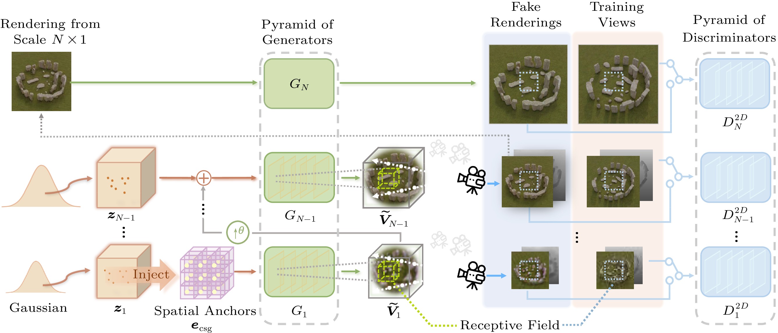
SinGRAV learns a powerful generative model for generating neural radiance volumes from multi-view observations $\mathcal{X} = \{ {\boldsymbol{x}}^1,\ldots, {\boldsymbol{x}}^m \}$ of a single scene, where $m$ denotes the viewpoint index. In contrast to learning class-specific priors, our specific aim is to learn the internal distribution of the input scene. To this end, we resort to a voxel-based neural scene representation, paired with convolutional generators, which inherently possess spatial locality bias, with limited receptive fields for learning over plenty of local regions. The generative model is learned via adversarial generation and discrimination through 2D projections of the generated volumes. During training, the camera pose is randomly selected from the training set. We will omit the notion of the camera pose for brevity. Overall, we use a multi-scale framework to learn properties at different scales ranging from global configurations to local fine texture details, and have to tackle the spatial geometric arrangement issues in 3D. Fig.2 presents an overview.

Figure  2.  SinGRAV training setup. A series of convolutional generators are trained to generate a scene in a coarse-to-fine manner. At each scale, $G_n$ learns to form a volume via generating realistic 3D overlapping patches, which collectively contribute to a volumetric-rendered imagery indistinguishable from the observation images of the input scene by the discriminator $D_n$. At the finest scale, the generator $G_N$ operates purely on the 2D domain to super-resolve the imagery produced from scale $N - 1$, significantly reducing the computation overhead. $\uparrow^{\theta}$ means volume upsampling.

下载: 全尺寸图片 幻灯片

3.1   Neural Radiance Volume and Rendering

The generated scene is represented by a discrete 3D voxel grid, and is to be produced by a 3D convolutional network. Each voxel center stores a 4-channel vector that contains a density scalar $\sigma$ and a color vector ${\boldsymbol{c}}$. Trilinear interpolation is used to define a continuous radiance field in the volume. We use the differentiable volume rendering^[15] to render images from generated volumes. Specifically, for each camera ray ${\boldsymbol{r}}$, the expected color $\hat{C}$ is approximated by integrating over $M$ samples spreading along the ray:

and $T_i = \exp\Big(-\sum_{j=1}^{i-1}\sigma _j \delta_j \Big),$ where the subscript denotes the sample index between the near $t_{\rm n}$ and far $t_{\rm f}$ bound, $\delta_i = t_{i+1} - t_i$ is the distance between two consecutive samples, and $T_i$ is the accumulated transmittance at sample $i$, which is obtained via integrating over the preceding samples along the ray. This function is differentiable and enables updating the volume based on the error derived from supervision signals.

Hybrid Multi-Scale Architecture. SinGRAV uses a hybrid multi-scale architecture that contains a generation pyramid with a hybrid use of 2D and 3D convolutional generators, and a discrimination pyramid inspecting local properties on 2D renderings at different scales.

3.1.1   Hybrid Generation Pyramid

There are a series of 3D convolutional generators $\{G_{ n}\}_{ n=1}^{N-1}$ and a lightweight 2D convolutional generator $G_N$ (see Fig.2). Overall, 3D generators at coarser scales learn to generate a radiance volume at an increasing resolution, and the volume resolution in the pyramid is increased by a factor of $\theta$ between two consecutive scales. At the $N$-th scale, to avoid the overly high computation issue, we use a lightweight 2D generator $G_N$ to directly super-resolve the rendering from the preceding scale by a factor ${\mu}_s$, achieving higher-resolution imagery. Importantly, these generators are equipped with limited receptive fields to capture the distribution of local patches, instead of memorizing the whole scene (i.e., reconstruction).

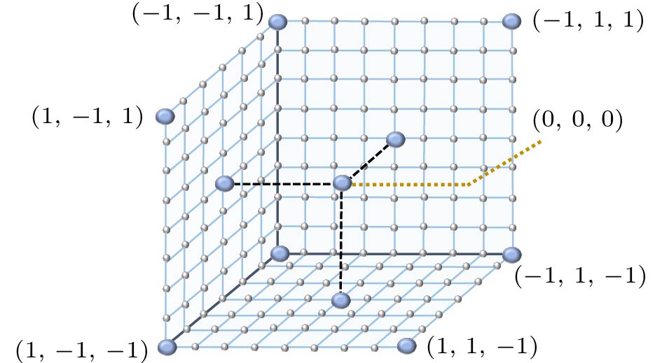
At the coarsest scale, the generation is produced in an unconditional manner, i.e., the radiance volume at the coarsest scale is purely generated from a Gaussian noise volume ${\boldsymbol{z}}_1$. Notably, we observe that learning the internal distribution with spatial-invariant and receptive field-limited convolutional networks leads to more difficulties in producing plausible 3D structures. Inspired by [32], which alleviates a similar issue in image generation by introducing spatial inductive bias, we introduce spatial inductive bias into our framework by using the 3D normalized Cartesian Spatial Grid (CSG):

where $W$, $H$, and $U$ are the size of the volume along the $x$-, $y$- and $z$-axis respectively. As illustrated in Fig.3, the grid is equipped with distinct spatial anchors, empowering the model with better spatial localization. The spatial anchors provided by ${\boldsymbol{e}}_\text{csg}$ are injected into the noise volume ${\boldsymbol{z}}_1$ at the coarsest level via an element-wise summation operation:

Figure  3.  Spatial anchors provided by ${\boldsymbol{e}}_\text{csg}$.

下载: 全尺寸图片 幻灯片

where ${ {\boldsymbol{z}}}_1,\: { {\boldsymbol{e}}}_\text{csg} \in \mathbb{R}^{3 \times U \times H \times W}$. Note we only inject the spatial inductive bias at the coarsest scale, as the positional-encoded information will be propagated through subsequent scales by convolution operations^[32]. The receptive field of $G_1$ is around $40\%$ of the volume of interest; thus $G_1$ learns to generate the overall layout.

Subsequently, $G_ n$ at finer scales ($1< n<N$) learns to add details missing from previous scales. Hence, each generator $G_ n$ takes as input a spatial noise volume ${\boldsymbol{z}}_ n$ and an upsampled volume of $({{\tilde{\boldsymbol{V}}}}_{ n-1}) \uparrow^{\theta}$ outputted from $G_{ n-1}$. Specially, prior to being fed into $G_ n$, ${\boldsymbol{z}}_ n$ is added to $({{\tilde{\boldsymbol{V}}}}_{ n-1}) \uparrow^{\theta}$, and, akin to residual learning^[41], $G_ n$ only learns to generate missing details:

At the finest scale, a 2D convolutional generator $G_N$ takes as input only the rendering ${{\tilde{\boldsymbol x}}}_{N-1}$ produced from $G_{N-1}$ and outputs a super-resolved image ${{\tilde{\boldsymbol x}}}_N$ with enhanced details:

$G_N$ utilizes upsampling layers introduced in [3], and produces the final image that is twice the resolution of ${{\tilde{\boldsymbol x}}}_{N-1}$.

3.1.2   Discrimination Pyramid

For supervising the generation at each scale, SinGRAV resorts to a pyramid of 2D discriminators that operate on 2D images obtained by volume-rendering the generated volume, instead of directly using expensive 3D convolutions. Specifically, at coarser scales $[1,{N-1}]$, discriminators $\{D_{ n}^{2D}\}_{ n=1}^{N-1}$ jointly discriminate on the RGB and depth renderings, of which the resolution between consecutive scales increases by a factor of ${\mu}_r$, to simultaneously inspect the texture and geometry. Although [18] also adopts joint discrimination on depth, their discriminator is to inspect the entire interior layout, while our $\{D_{ n}^{2D}\}_{ n=1}^{N-1}$ is to learn plausible geometric arrangements from local patches. At the finest scale, where the input is an RGB image directly generated from the generator, to improve the view consistency, we adopt the dual discrimination strategy as in [2] for the discriminator $D_N^{2D}$ by concatenating the naively super-resolved $( {{\tilde{\boldsymbol x}}}_{N-1})\uparrow^{\mu_s}$ with the output from $G_{N}$. Overall, to progressively learn the internal priors, the receptive field of $D_{ n}^{2D}$ is so limited that local regions in the generated scene can be gradually crafted.

3.2   Training Loss

The multi-scale architecture is sequentially trained, from the coarsest to the finest scale. We construct a pyramid of resized input observations, $\mathcal{X}_ n = \{ {\boldsymbol{x}}_{ n} \}_{ n=1}^{N}$, for providing supervisions. The GANs at coarser scales are frozen once trained. The training objective is as follows:

where $\mathcal{L}_\text{adv}$ is an adversarial term, $\mathcal{L}_\text{rec}$ is a reconstruction term as similar in [6], $\mathbb{1}(\cdot)$ is an indicator function to activate the associated term iff the condition is satisfied, and $\mathcal{L}_\text{swd}$ calculates the Sliced Wasserstein Distance (SWD) as in [42]. SWD measures the distance between the textural distributions of two images, while neglecting the difference of the global layouts. Concretely, $\mathcal{L}_\text{swd}$ is given by: $\mathcal{L}_\text{swd} = \mathcal{L}_\text{swd}({\boldsymbol{x}}_N, {{\tilde{\boldsymbol x}}}_N) = \sum_{k=1}^{K} \mathcal{L}_\text{swd}(\tilde{\boldsymbol{f}}^{\:k}, \boldsymbol{f}^{\:k})$, where $\tilde{\boldsymbol{f}}^{\:k}$ and $\boldsymbol{f}^{\:k}$ are features from layer $k$ of a pre-trained VGG-19 network^[43] (please refer to [42] for more details). In the following, we elaborate the designs of $\mathcal{L}_\text{adv}$ and $\mathcal{L}_\text{rec}$.

3.2.1   Adversarial Loss

We use the WGAN-GP loss^[44] as $\mathcal{L}_\text{adv}$ for stabilizing the training. The discrimination score is obtained by averaging over the patch discrimination map of $D_{ n}^{2D}$. During training, we render the depth from the generated volume, and concatenate the depth and color images for the input to $\{D_{ n}^{2D}\}_{n=1}^{N-1}$ as fake samples, while real samples for depth can be derived with multi-view geometry techniques trivially. For preparing the real input to discriminator $D_{N}^{2D}$, we upsample the resized observation ${\boldsymbol{x}}_{N-1}$ via bilinear upsampling and concatenate the upsampled image with the ground truth observation ${ {\boldsymbol{x}}}_N$.

3.2.2   Reconstruction Loss

Inspired by [6], we introduce a specific set of input noise volumes to ensure that they can reconstruct the underlying scene depicted in the observations $\mathcal{X}$. Specifically, a set of fixed noise volumes are defined as $\{ {\boldsymbol{z}}_{ n}^{*}\}_{ n=1}^{N-1} = \{ {\boldsymbol{z}}_{1}^{*}, 0,\ldots, 0\}$. The reconstructed radiance volumes and associated renderings are denoted as $\{ {\boldsymbol{V}}_{ n}^{*}\}_{ n=1}^{N-1}$ and $\{ {{\tilde{\boldsymbol x}}}_{ n}^{*}, \tilde{{\boldsymbol{\boldsymbol{d}}}}_{ n}^{*}\}_{ n=1}^{N}$, respectively. Then the reconstruction loss $\mathcal{L}_\text{rec}$ is defined as:

where $\lambda_c$ and $\lambda_d$ are balance parameters and we set $\lambda_c=10$ and $\lambda_d=30$. As shown in (1), we use supervisions on both color images and depth images for achieving higher quality. Note that the depth penalty term is removed at the last scale since $G_N$, which only works in the color image domain. As demonstrated and discussed later in Subsection 4.4.2, our method can be applied even in cases where ground-truth depth maps are unavailable. In such scenarios, reconstructed depth maps generated by NeRF^[15] models or our proposed framework can be utilized.

4.   Experiments

4.1   Settings

4.1.1   Data

To evaluate the proposed framework, we collect observation images from a dozen of diverse scenes, which exhibit ample variations over the global arrangements and constituents. Specifically, we collect 3D scene assets from this website ², under TurboSquid 3D Model License ³. For eliminating the influence of data defects including incorrect camera pose estimation, incomplete scene coverage within the multi-view images, etc., we use rendered multi-view images in our main experiments, comparison experiments, and ablation study. Specifically, we utilize the path-tracing renderer in Blender to get the multi-view RGB-D observation. For data rendering, we scale the scenes so that the volume of interest stays within a cube with side width = $2$ (within the range $[-1, 1]$). Finally, for each scene, we render 200 observation images that fully cover the scene, for which the camera positions are randomly sampled on a hemisphere. Random natural scene generation of our method is demonstrated upon all collected scenes, whereas more evaluations are conducted on a subset (stonehenge, grass and flowers, and island).

Moreover, in Subsection 4.5, we test our framework on captured data obtained by a hand-hold phone. For captured multi-view images, we utilize COLMAP to reconstruct camera poses, which is a common practice in many neural scene representation frameworks^{[15, 45]}.

4.1.2   Evaluation Measures

We extend common metrics in single image generation to quantitatively assess $m=50$ scenes generated from each input scene. For each generated scene, $k=40$ images at random viewpoints are rendered for evaluation under a multi-view setting: 1) SIFID-MV measures how well the model captures the internal statistics of the input by SIFID^[6] averaged over multi-view images of a generated scene; 2) Diversity-MV measures the diversity of generated scenes by the averaged image diversity^[6] over multiple views.

4.2   Neural Scene Variations

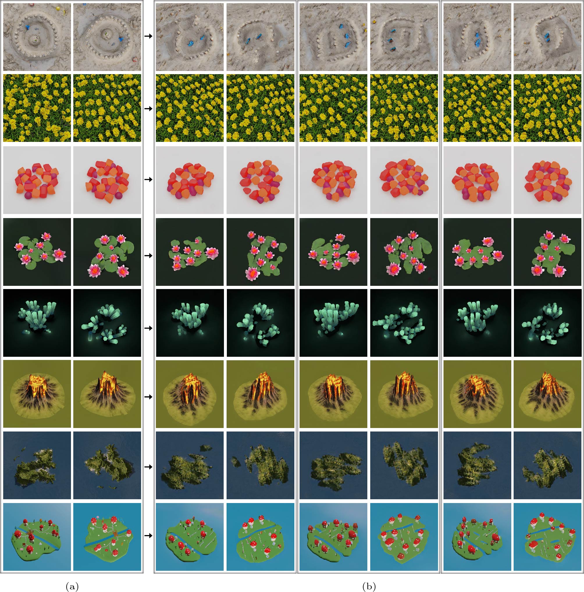
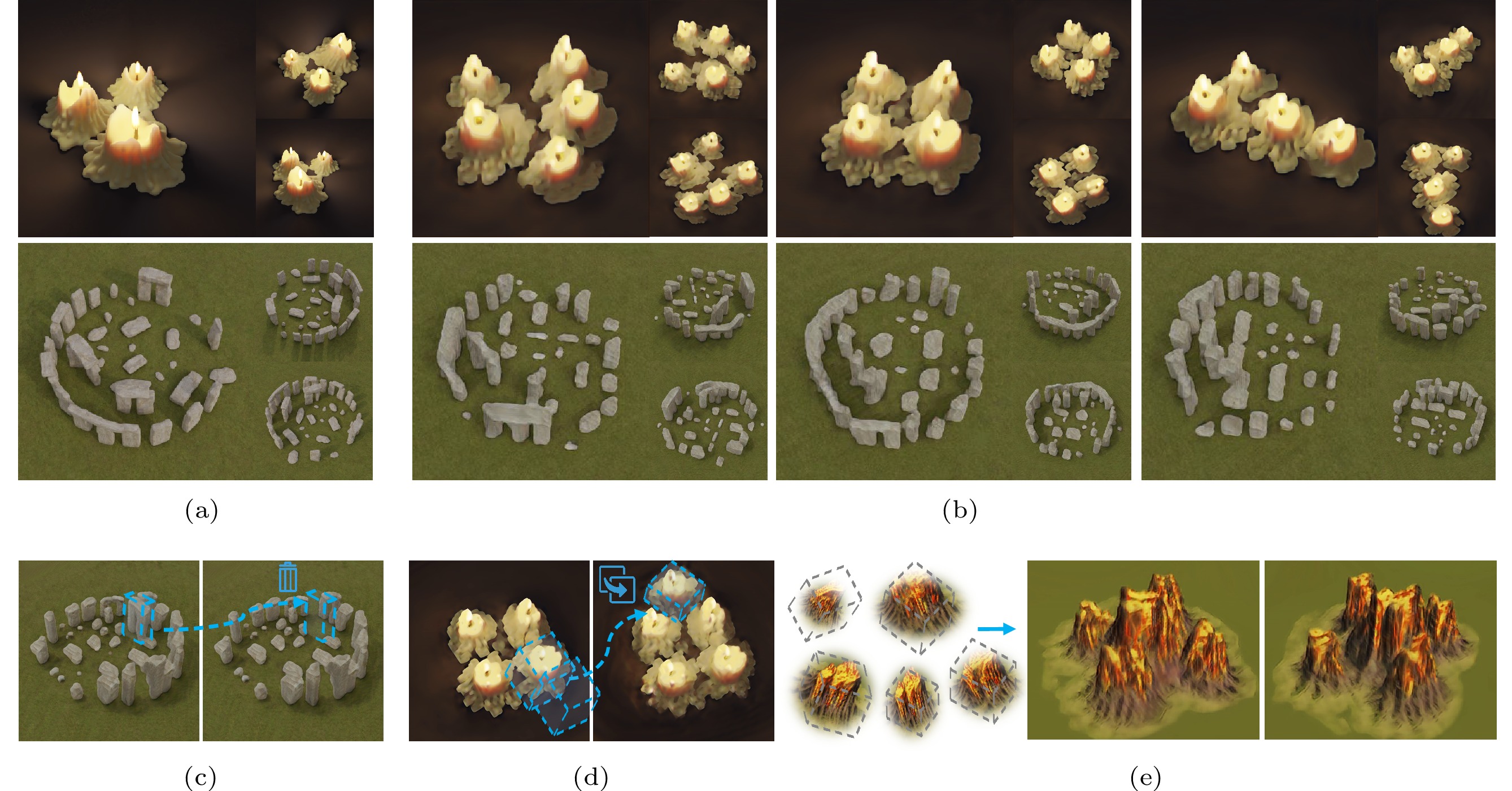
Fig.1 and Fig.4 present qualitative results of SinGRAV, where the generated scenes depict reasonably new global layouts, and objects with various shapes and realistic looking. These results suggest the efficacy of SinGRAV in modeling the internal patch distribution within the input scene. On grass and flowers exhibiting uniform yet complicated textures over an open field, SinGRAV produces high-quality random generation results. Moreover, SinGRAV is able to capture the global illumination to some extent, as evidenced by the shadows around stones and islands, along with the illumination changes under spinning cameras on samples of mushroom. In Fig.5, we demonstrate examples for extracted meshes of the generated scenes from SinGRAV, which demonstrate the ability to capture the geometric distribution of the exemplar scene. In addition, we present more visual results in the supplementary video ⁴.

Figure  4.  Random scene generation. (a) Sampled views for different training scenes. (b) Rendered views from three randomly generated scenes. In each row, the images shown in (a) and (b) are under the same viewpoints. After training on multi-view observations of an input scene, SinGRAV learns to generate similar scenes with new objects and configurations. Note the observation images of the beach castle at the top row are taken from the real world, and novel beach castles with various layouts are generated by SinGRAV.

下载: 全尺寸图片 幻灯片

Figure  5.  Examples for extracted meshes from generated scenes produced by SinGRAV.

下载: 全尺寸图片 幻灯片

4.3   Comparisons

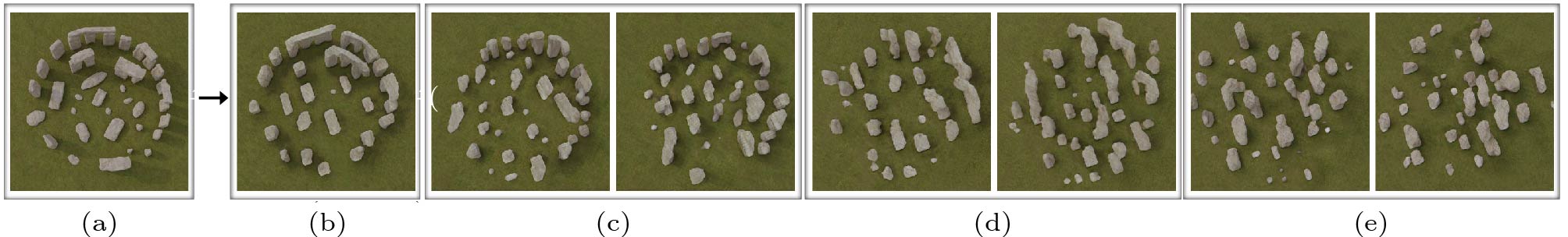
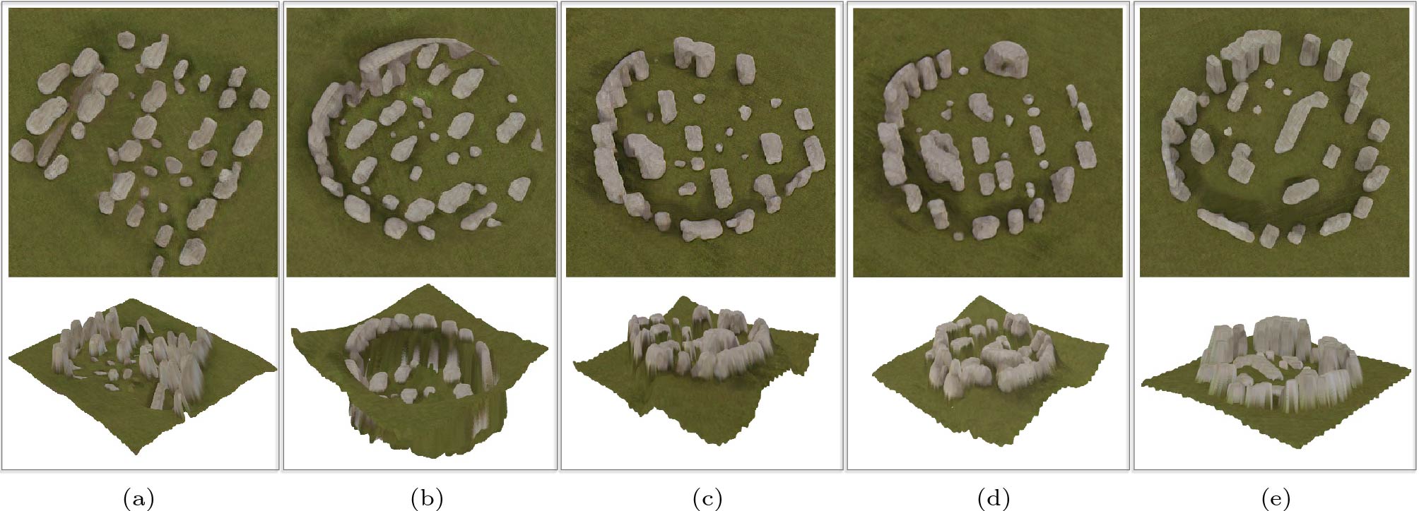
We compare our framework SinGRAV with three state-of-the-art neural scene generative models, namely, GRAF^[4], pi-GAN^[1], and GIRAFFE^[5]. We use their official codes for training these baselines. Training details of each baseline can be found in the supplementary material ⁵. For fair comparisons, similar to SinGRAV, we use ground truth cameras when training baselines, instead of using random cameras from a predefined camera distribution. The quantitative and qualitative results are presented in Table 1 and Fig.6, respectively. Table 1 shows that pi-GAN produces the best SIFID-MV score, but the value of Diversity-MV drastically degrades. GRAF and GIRAFFE also exhibit a significantly degraded diversity score. Qualitative results in Fig.6 show that these baselines suffer from severe mode collapse, due to the lack of diverse samples for learning category-level priors.

Table  1.  Quantitative Comparisons

Method	Img. Res.	SIFID-MV $\downarrow$	Diversity-MV $\uparrow$
GRAF[4]	$320\times320$	0.4447	0.1337
pi-GAN[1]	$128\times128$	0.0133	0.1157
GIRAFFE[5]	$320\times320$	0.4710	0.3198
SinGRAV	$320\times320$	0.1113	0.7769
Note: The top two on each metric are bolded. All baselines suffer from severe mode collapse, producing low Diversity-MV scores. Img. Res.: image resolution. $\downarrow$: the lower, the better; $\uparrow$: the higher, the better.

下载: 导出CSV 

| 显示表格

Figure  6.  Qualitative results for comparisons. (a) Training scenes. (b) Randomly generated scenes from GRAF^[4]. (c) Randomly generated scenes from pi-GAN^[1]. (d) Randomly generated scenes from GIRAFFE^[5]. (e) Randomly generated scenes from SinGRAV. All baselines encounter severe mode-collapse issues, while SinGRAV generates diverse samples.

下载: 全尺寸图片 幻灯片

4.4   Validation of Design Choices

We conduct experiments to evaluate several key design choices and the quantitative results are reported in Table 2.

Table  2.  Numerical Results for Variants of SinGRAV

Variant	Img. Res.	SIFID-MV $\downarrow$	Diversity-MV $\uparrow$
(wo. CSG)	$320^2$	0.1307	0.8434
(wo. depth sup.)	$320^2$	0.1157	0.7910
(NeRF-depth)	$320^2$	0.1290	0.8046
(self-depth)	$320^2$	0.1120	0.7862
(wo. SWD)	$320^2$	0.2713	0.7730
(w. MLP)	$160^2$	0.1843	0.5235
(w. MLP-LLG)	$108^2$	0.2013	0.4621
SinGRAV	$320^2$	0.1113	0.7769
Note: wo.: without; w.: with.

下载: 导出CSV 

| 显示表格

4.4.1   Spatial Inductive Bias

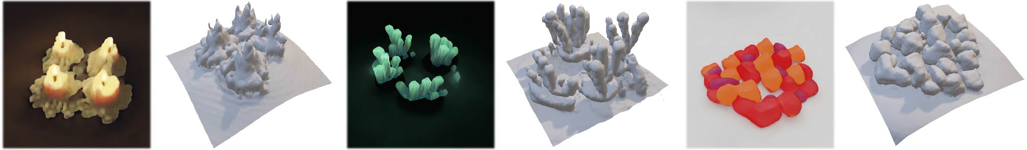
We build a variant—SinGRAV (wo. CSG), which is trained without the spatial anchor volume ${\boldsymbol{e}}_\text{csg}$. As shown in Table 2, compared with SinGRAV, SinGRAV (wo. CSG) produces a worse SIFID-MV score (increased by $17\%$) and an increased Diversity-MV score. While the latter suggests increased diversity, we observe from the visual results that the spatial arrangements of objects deviate significantly from that of the input, producing floating stones, as shown in Fig.7(a).

Figure  7.  Influence of spatial inductive bias and depth supervision strategies. (a) Results from SinGRAV (wo. CSG). (b) Results from SinGRAV (wo. depth sup.). (c) Results from SinGRAV (NeRF-depth). (d) Results from SinGRAV (self-depth). (e) Results from SinGRAV with GT depth. One generated sample with the corresponding point cloud is shown in (a)–(e). Without the inductive bias or depth supervision, the generated scenes exhibit implausible geometric structures, while the variants that use reconstructed depth maps or ground-truth depth preserve the spatial arrangement well.

下载: 全尺寸图片 幻灯片

4.4.2   Depth Supervision Strategy

To investigate the role exerted by the depth supervision (depth sup.) and the influence of using reconstructed depth cues, we conduct experiments on three variants of SinGRAV, including SinGRAV (wo. depth sup.), SinGRAV (self-depth) and SinGRAV (NeRF-depth).

In the first variant, SinGRAV (wo. depth sup.), we remove the depth supervisions and present the numerical results in Table 2. Visual results are also provided in Fig.7. While the numerical results for this variant are comparable to those of our full model SinGRAV, Fig.7 shows that the extracted point clouds exhibit undesirable geometric structures in the generated scenes of SinGRAV (wo. depth sup.). Additionally, in the supplementary video ⁶, we include multi-view videos to further illustrate the suboptimal geometry produced by this variant. These results emphasize the importance of incorporating depth supervisions during the training.

There are many scenarios where perfect ground-truth depth is not available; thus we further investigate the feasibility of utilizing reconstructed depth information from multi-view RGB images. The variant SinGRAV (NeRF-depth) uses the depth obtained from a NeRF^[15] reconstruction of the input scene, and SinGRAV (self-depth) uses the depth obtained from the reconstructed volume with ${\boldsymbol{z}}^*$ from our framework trained with $\lambda_d = 0$. Table 2 shows that SinGRAV (NeRF-depth) and SinGRAV (self-depth) are able to achieve comparable performance to SinGRAV, implying that SinGRAV is robust to the quality of the depth data. The extracted point clouds from generated scenes, as shown in Fig.7, also demonstrate that using depth supervision coming from reconstructed depth can generate reasonable geometric arrangements. Furthermore, we provide multi-view videos of the generated scenes from two aforementioned variants for enhanced visualization. To encapsulate, depth data obtained via reconstruction methods suffice to guide the learning of global geometric structures, reinforcing the adaptability and versatility of SinGRAV in diverse scenarios.

4.4.3   SWD Loss

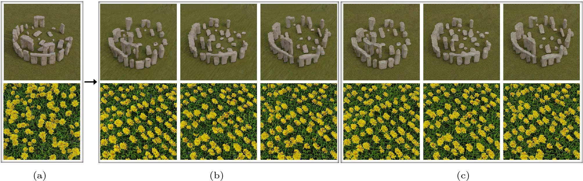
If $\mathcal{L}_\text{swd}$ is eliminated, the internal distribution of generated scenes would differ greatly from that of the input, leading to significantly increased SIFID-MV at the fifth row (wo. SWD) in Table 2. Correspondingly, the visual results in Fig.8 also show that SinGRAV(wo. $\mathcal{L}_\text{swd}$) produces blurry and less realistic textures, suggesting the efficacy of $\mathcal{L}_\text{swd}$ in improving visual quality.

Figure  8.  SinGRAV vs SinGRAV (wo. $\mathcal{L}_\text{swd}$). (a) Two training scenes. (b) Rendered results of generated scenes from SinGRAV (wo. $\mathcal{L}_\text{swd}$). (c) Rendered results of generated scenes from SinGRAV. Without the SWD loss at the finest scale, SinGRAV (wo. $\mathcal{L}_\text{swd}$) produces blurry textures and undesired artifacts, while training with SWD loss significantly improves the texture quality.

下载: 全尺寸图片 幻灯片

4.4.4   MLP vs Voxel

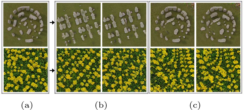
To validate our choice of adopting the voxel-based representation, we design a variant SinGRAV (w. MLP), which integrates a conditional MLP-based radiance field as in [4]. The numerical results of SinGRAV (w. MLP), which uses a conditional MLP-based radiance field as in GRAF, are reported in Table 2. The highest image resolution is $160\times160$ due to overly high memory consumption. SinGRAV (w. MLP) degrades in both the quality and diversity, which is also reflected by the visuals in Fig.2. Note that, although the same patch discrimination strategy is used, SinGRAV (w. MLP) suffers from severe mode collapse. We believe this is because the generative output of coordinate-based MLPs is very likely to be dominated by the input coordinates. The poor generation is also possibly a product of the conflict between the lack of locality in the fully-connected layers^[8] and the limited receptive field in the adversarial training. In addition, we train a variant SinGRAV (w. MLP-LLG), which incorporates a local latent grid (LLG) proposed in [18] to increase the capacity of the MLP-based representation. Fig.9 shows that the generated layouts are improved with the increased locality; however, severe mode collapse still exists. On the other hand, we believe more efforts can be made in the future to adapt MLP-based representations for our task.

Figure  9.  Qualitative results of using MLP-based representations. (a) Training scenes. (b) Generated scenes from SinGRAV (w. MLP). (c) Generated scenes from SinGRAV (w. MLP-LLG). SinGRAV (w. MLP) produces grid patterns, which are alleviated by the use of local latent grid in SinGRAV (w. MLP-LLG). Nevertheless, both variants suffer from severe mode collapse, and generate almost identical scene samples.

下载: 全尺寸图片 幻灯片

4.4.5   Influence of Varying Pyramid Depth

We train variants with various numbers of scales. Specifically, for training a variant with $t$ ($t < N$) scales, we use generators $\{G_{ n}\}_{ n=N-t+1}^N$ and discriminators $\{D_{ n}^{2D}\}_{ n=N-t+1}^N$ to preserve the final image resolution. As shown in Fig.10, with less scales, the effective receptive field at the coarsest scale is rather small, resulting in a model that only captures local properties, whereas, using more scales allows modeling plausible global arrangements.

Figure  10.  Influence of different numbers of scales. (a) Training scene. (b) Generated scene from SinGRAV with $N=6$. (c) Generated scenes from SinGRAV with $N=5$. (c) Generated scenes from SinGRAV with $N=4$. (e) Generated scenes from SinGRAV with $N=3$. Training with more scales is beneficial to the modeling of global arrangements, while a model with less scales tends to capture only local textures. $N$ is set to $6$ by default for SinGRAV.

下载: 全尺寸图片 幻灯片

4.5   Results on Real-World Data

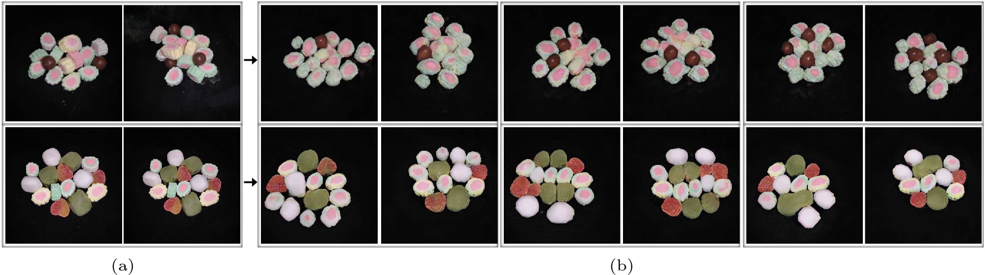
To investigate the applicability of SinGRAV on real-world data, we test SinGRAV on a daily scenario where people use a mobile phone to capture multi-view images of a desktop scene. Specifically, we capture dozens of images of two candy piles. The flash is turned on for removing the shadows introduced by the hands and the hand-hold devices. Then we use COLMAP to estimate the camera poses of the captured images. Once the poses are estimated, we adopt MultiNeRF ⁷ to reconstruct the captured scene. Finally, given the MultiNeRF-parameterized scene, we can render multi-view images with roughly consistent camera-scene distances for training SinGRAV. Since the ground-truth depth maps are not available for images captured by hand-hold phones, we use rendered depth maps from the reconstructed scene to train our framework.

The generated scenes are shown in Fig.11. As shown in Fig.11, SinGRAV is able to produce plausible scenes with considerable diversity, demonstrating the applicability of SinGRAV on real-world captured images. The results further manifest that the proposed framework can achieve appealing results by using reconstructed depth maps from multi-view images. The rendered multi-view observations from more generated scenes can be found in the supplementary video ⁸.

Figure  11.  Random scene samples generated from two real-world indoor scenes. (a) Two views of the training scenes. (b) Three randomly generated scenes from SinGRAV separately trained on the training scenes. Each scene is rendered with the same two views.

下载: 全尺寸图片 幻灯片

4.6   Applications

SinGRAV supports various applications, which can be achieved by naively manipulating generated volumes at coarse scales and using subsequent generators to harmonize the modifications. Specifically, we derive three applications with SinGRAV, including 3D scene editing with removal and duplicate operations, composition, and animation. Fig.1 presents the results. More results and implementation details are given in the supplementary material ⁹.

5.   Conclusions

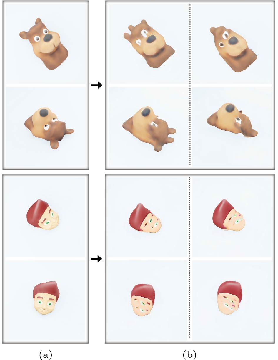
In this work, we made an attempt to learn a deep generative neural scene model from visual observations of a single scene. Once trained on a single scene, the model can generate novel scenes with plausible geometries and arrangements, which can be rendered with pleasing viewing effects. The importance of key design choices is validated. Despite successful demonstrations, our proposed SinGRAV has a few limitations. While SinGRAV learns from a single scene, bypassing the need for collecting data from many homogeneous 3D samples, multi-view images with sufficient coverage rate of the scene are yet required. Moreover, albeit validated, the use of voxel grids inherently limits the network capacity in modeling fine details, consequently hindering the model from achieving high-resolution imagery. Our remedy is to incorporate a 2D neural renderer that operates on the 2D domain to super-resolve the imagery, which inevitably introduces the multi-view inconsistency. There are view inconsistencies in complex textural areas, e.g., the thin structures in the grass and flowers scene. A future direction would be to overturn this design, with more endeavors on exploiting MLP-based representations to model continuous volumes. We also noticed that, when the exemplar scene is dominant by a structure-sensitive object, as demonstrated in Fig.12, SinGRAV may produce less satisfying results. Besides, the proposed method, in its current form, sometimes produces artifacts in the background, as it does not incorporate special designs for modeling the background. Hence, it would also be worth addressing this issue, especially for scenes with complicated backgrounds, potentially with special considerations on the foreground-background continuity.

Figure  12.  Results for structure-sensitive object-centric scenes. (a) Two training scenes. (b) Randomly generated scenes from SinGRAV. When the exemplar scene is predominantly occupied by a single object, SinGRAV possibly produces less satisfying results due to the insufficiency of exploitable patch priors and unawareness of the underlying semantics.

下载: 全尺寸图片 幻灯片